Note
Go to the end to download the full example code or to run this example in your browser via Binder
Time series#
Interpolation of a time series
This example shows how to interpolate a time series using the library.
Note
This example is not executed because it needs to access data in the e-cloud. But you can run it on binder.
In this example, we consider the time series of MSLA maps distributed by AVISO/CMEMS. We start by retrieving the data:
import datetime

import cartopy.crs
import cartopy.feature
import intake
import matplotlib.pyplot
import numpy
import pandas

import pyinterp.backends.xarray
import pyinterp.tests

cat = intake.open_catalog('https://raw.githubusercontent.com/pangeo-data'
                          '/pangeo-datastore/master/intake-catalogs/'
                          'ocean.yaml')
ds = cat['sea_surface_height'].to_dask()
To manage the time series retrieved, we create the following object:
class TimeSeries:
    """Manage a time series composed of a grid stack."""

    def __init__(self, ds):
        self.ds = ds
        self.series, self.dt = self._load_ts()

    @staticmethod
    def _is_sorted(array):
        indices = numpy.argsort(array)
        return numpy.all(indices == numpy.arange(len(indices)))

    def _load_ts(self):
        """Loading the time series into memory."""
        time = self.ds.time
        assert self._is_sorted(time)

        series = pandas.Series(time)
        frequency = set(
            numpy.diff(series.values.astype('datetime64[s]')).astype('int64'))
        if len(frequency) != 1:
            raise RuntimeError(
                'Time series does not have a constant step between two '
                f'grids: {frequency} seconds')
        return series, datetime.timedelta(seconds=float(frequency.pop()))

    def load_dataset(self, varname, start, end):
        """Loading the time series into memory for the defined period.

        Args:
            varname (str): Name of the variable to be loaded into memory.
            start (datetime.datetime): Date of the first map to be loaded.
            end (datetime.datetime): Date of the last map to be loaded.

        Returns:
            pyinterp.backends.xarray.Grid3D: The interpolator handling the
            interpolation of the grid series.
        """
        if start < self.series.min() or end > self.series.max():
            raise IndexError(
                f'period [{start}, {end}] out of range [{self.series.min()}, '
                f'{self.series.max()}]')
        first = start - self.dt
        last = end + self.dt

        selected = self.series[(self.series >= first) & (self.series < last)]
        print(f'fetch data from {selected.min()} to {selected.max()}')

        data_array = ds[varname].isel(time=selected.index)
        return pyinterp.backends.xarray.Grid3D(data_array)


time_series = TimeSeries(ds)
The test data set containing a set of positions of different floats is then loaded.
def cnes_jd_to_datetime(seconds):
    """Convert a date expressed in seconds since 1950 into a calendar date."""
    return datetime.datetime.utcfromtimestamp(
        ((seconds / 86400.0) - 7305.0) * 86400.0)


def load_positions():
    """Loading and formatting the dataset."""
    df = pandas.read_csv(pyinterp.tests.positions_path(),
                         header=None,
                         sep=r';',
                         usecols=[0, 1, 2, 3],
                         names=['id', 'time', 'lon', 'lat'],
                         dtype=dict(id=numpy.uint32,
                                    time=numpy.float64,
                                    lon=numpy.float64,
                                    lat=numpy.float64))
    df.mask(df == 1.8446744073709552e+19, numpy.nan, inplace=True)
    df['time'] = df['time'].apply(cnes_jd_to_datetime)
    df.set_index('time', inplace=True)
    df['sla'] = numpy.nan
    return df.sort_index()


df = load_positions()
Two last functions are then implemented. The first function will divide the time series to be processed into weeks.
def periods(df, time_series, frequency='W'):
    """Return the list of periods covering the time series loaded in memory."""
    period_start = df.groupby(
        df.index.to_period(frequency))['sla'].count().index

    for start, end in zip(period_start, period_start[1:]):
        start = start.to_timestamp()
        if start < time_series.series[0]:
            start = time_series.series[0]
        end = end.to_timestamp()
        yield start, end
    yield end, df.index[-1] + time_series.dt
The second one will interpolate the DataFrame loaded in memory.
def interpolate(df, time_series, start, end):
    """Interpolate the time series over the defined period."""
    interpolator = time_series.load_dataset('sla', start, end)
    mask = (df.index >= start) & (df.index < end)
    selected = df.loc[mask, ['lon', 'lat']]
    df.loc[mask, ['sla']] = interpolator.trivariate(
        dict(longitude=selected['lon'].values,
             latitude=selected['lat'].values,
             time=selected.index.values),
        interpolator='inverse_distance_weighting',
        num_threads=0)
Finally, the SLA is interpolated on all loaded floats.
for start, end in periods(df, time_series, frequency='M'):
    interpolate(df, time_series, start, end)
Visualization of the SLA for a float.
float_id = 62423050
selected_float = df[df.id == float_id]
first = selected_float.index.min()
last = selected_float.index.max()
size = (selected_float.index - first) / (last - first)
fig = matplotlib.pyplot.figure(figsize=(10, 5))
ax = fig.add_subplot(111,
                     projection=cartopy.crs.PlateCarree(central_longitude=180))
sc = ax.scatter(selected_float.lon,
                selected_float.lat,
                s=size * 100,
                c=selected_float.sla,
                transform=cartopy.crs.PlateCarree(),
                cmap='jet')
ax.coastlines()
ax.set_title('Time series of SLA '
             '(larger points are closer to the last date)')
ax.add_feature(cartopy.feature.LAND)
ax.add_feature(cartopy.feature.COASTLINE)
ax.set_extent([80, 100, 13.5, 25], crs=cartopy.crs.PlateCarree())
fig.colorbar(sc)
The image below illustrates the result of the code above:
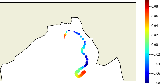
Time series of SLA observed by float #62423050 (larger points are closer to the last date)#