2D interpolation

Interpolation of a two-dimensional regular grid.

Bivariate

Perform a bivariate interpolation of gridded data points.

import cartopy.crs
import matplotlib
import matplotlib.pyplot
import numpy

import pyinterp
import pyinterp.backends.xarray
import pyinterp.tests

The first step is to load the data into memory and create the interpolator object:

Note

An exception will be thrown if the constructor is not able to determine which axes are the longitudes and latitudes. You can force the data to be read by specifying on the longitude and latitude axes the respective degrees_east and degrees_north attribute units. If your grid does not contain geodetic coordinates, set the geodetic option of the constructor to False.

ds = pyinterp.tests.load_grid2d()
interpolator = pyinterp.backends.xarray.Grid2D(ds.mss)

We will then build the coordinates on which we want to interpolate our grid:

Note

The coordinates used for interpolation are shifted to avoid using the points of the bivariate function.

mx, my = numpy.meshgrid(numpy.arange(-180, 180, 1) + 1 / 3.0,
                        numpy.arange(-89, 89, 1) + 1 / 3.0,
                        indexing='ij')

The grid is interpolated to the desired coordinates:

mss = interpolator.bivariate(
    coords=dict(lon=mx.ravel(), lat=my.ravel())).reshape(mx.shape)

Let’s visualize the original grid and the result of the interpolation.

fig = matplotlib.pyplot.figure(figsize=(10, 8))
ax1 = fig.add_subplot(
    211, projection=cartopy.crs.PlateCarree(central_longitude=180))
lons, lats = numpy.meshgrid(ds.lon, ds.lat, indexing='ij')
pcm = ax1.pcolormesh(lons,
                     lats,
                     ds.mss.T,
                     cmap='jet',
                     shading='auto',
                     transform=cartopy.crs.PlateCarree(),
                     vmin=-0.1,
                     vmax=0.1)
ax1.coastlines()
ax1.set_title('Original MSS')
ax2 = fig.add_subplot(212, projection=cartopy.crs.PlateCarree())
pcm = ax2.pcolormesh(mx,
                     my,
                     mss,
                     cmap='jet',
                     shading='auto',
                     transform=cartopy.crs.PlateCarree(),
                     vmin=-0.1,
                     vmax=0.1)
ax2.coastlines()
ax2.set_title('Bilinear Interpolated MSS')
fig.colorbar(pcm, ax=[ax1, ax2], shrink=0.8)
fig.show()

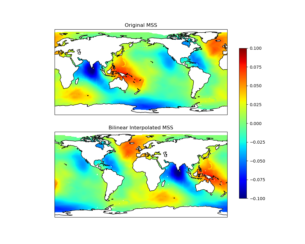
Values can be interpolated with several methods: bilinear, nearest, and inverse distance weighting. Distance calculations, if necessary, are calculated using the Haversine formula.

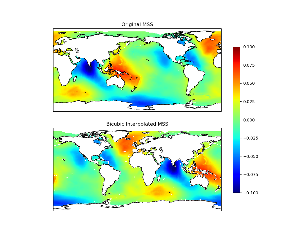
Bicubic

To interpolate data points on a regular two-dimensional grid. The interpolated surface is smoother than the corresponding surfaces obtained by bilinear interpolation. Spline functions provided by GSL achieve bicubic interpolation.

Warning

When using this interpolator, pay attention to the undefined values. Because as long as the calculation window uses an indefinite point, the interpolator will compute indeterminate values. In other words, this interpolator increases the area covered by the masked values. To avoid this behavior, it is necessary to pre-process the grid to delete undefined values.

The interpolation bicubic function has more parameters to define the data frame used by the spline functions and how to process the edges of the regional grids:

mss = interpolator.bicubic(coords=dict(lon=mx.ravel(), lat=my.ravel()),
                           nx=3,
                           ny=3).reshape(mx.shape)

Warning

The grid provided must have strictly increasing axes to meet the specifications of the GSL library. When building the grid, specify the increasing_axes option to flip the decreasing axes and the grid automatically. For example:

interpolator = pyinterp.backends.xarray.Grid2D(
    ds.mss, increasing_axes=True)

fig = matplotlib.pyplot.figure(figsize=(10, 8))
ax1 = fig.add_subplot(
    211, projection=cartopy.crs.PlateCarree(central_longitude=180))
pcm = ax1.pcolormesh(lons,
                     lats,
                     ds.mss.T,
                     cmap='jet',
                     shading='auto',
                     transform=cartopy.crs.PlateCarree(),
                     vmin=-0.1,
                     vmax=0.1)
ax1.coastlines()
ax1.set_title('Original MSS')
ax2 = fig.add_subplot(212, projection=cartopy.crs.PlateCarree())
pcm = ax2.pcolormesh(mx,
                     my,
                     mss,
                     cmap='jet',
                     shading='auto',
                     transform=cartopy.crs.PlateCarree(),
                     vmin=-0.1,
                     vmax=0.1)
ax2.coastlines()
ax2.set_title('Bicubic Interpolated MSS')
fig.colorbar(pcm, ax=[ax1, ax2], shrink=0.8)
fig.show()