Unstructured grid

Interpolation of unstructured grids.

The interpolation of this object is based on a R*Tree structure. To begin with, we start by building this object. By default, this object considers the WGS-84 geodetic coordinate system. But you can define another one using the class Spheroid.

import matplotlib.pyplot
import numpy

import pyinterp

mesh = pyinterp.RTree()

Then, we will insert points into the tree. The class allows you to add points using two algorithms. The first one called packing, will enable you to enter the values in the tree at once. This mechanism is the recommended solution to create an optimized in-memory structure, both in terms of construction time and queries. When this is not possible, you can insert new information into the tree as you go along using the insert method.

SIZE = 2000
X0, X1 = 80, 170
Y0, Y1 = -45, 30
lons = numpy.random.uniform(low=X0, high=X1, size=(SIZE, ))
lats = numpy.random.uniform(low=Y0, high=Y1, size=(SIZE, ))
data = numpy.random.uniform(low=-1.0, high=1.0, size=(SIZE, ))

Populates the search tree

mesh.packing(numpy.vstack((lons, lats)).T, data)

When the tree is created, you can interpolate data with four algorithms:

• Inverse Distance Weighting or IDW

• Radial Basis Function or RBF

• Window Function

• Universal Kriging

Inverse Distance Weighting (IDW), Radial Basis Function (RBF), and Kriging are all interpolation methods used to estimate a value for a target location based on the values of surrounding sample points. However, each method approaches this estimation differently.

IDW uses a weighted average of the surrounding sample points, where the weight assigned to each point is inversely proportional to its distance from the target location. The further away a sample point is from the target location, the less influence it has on the estimated value. This method is relatively simple to implement and computationally efficient, but it can produce over-smoothed results in areas with a lot of sample points and under-smoothed results in areas with few sample points.

RBF, on the other hand, models the spatial relationship between sample points and the target location by using a mathematical function (radial basis function) that is based on the distance between the points. The radial basis function is usually Gaussian, multiquadric, or inverse multiquadric. The estimated value at the target location is obtained by summing up the weighted contributions of all sample points. This method is more flexible than IDW as it can produce a wide range of interpolation results, but it can also be computationally expensive and susceptible to overfitting if not implemented carefully.

Kriging, also known as Gaussian process regression, is a geostatistical method that models the spatial structure of the underlying data by using a covariance matrix. The estimated value at the target location is obtained by solving a set of linear equations that balance the fit to the sample points and the smoothness of the estimated surface. Kriging can produce more accurate results than IDW and RBF in many cases, but it requires a good understanding of the spatial structure of the data and can be computationally demanding.

In summary, IDW is a simple and computationally efficient method, RBF is flexible but can be susceptible to overfitting, and Kriging is more accurate but requires a good understanding of the spatial structure of the data. The choice of method depends on the nature of the data, the spatial resolution required, and the computational resources available.

We start by interpolating using the IDW method

STEP = 1 / 32
mx, my = numpy.meshgrid(numpy.arange(X0, X1 + STEP, STEP),
                        numpy.arange(Y0, Y1 + STEP, STEP),
                        indexing='ij')

idw, neighbors = mesh.inverse_distance_weighting(
    numpy.vstack((mx.ravel(), my.ravel())).T,
    within=False,  # Extrapolation is forbidden
    k=11,  # We are looking for at most 11 neighbors
    num_threads=0)
idw = idw.reshape(mx.shape)

Interpolation with RBF method

rbf, neighbors = mesh.radial_basis_function(
    numpy.vstack((mx.ravel(), my.ravel())).T,
    within=False,  # Extrapolation is forbidden
    k=11,  # We are looking for at most 11 neighbors
    rbf='linear',
    smooth=1e-4,
    num_threads=0)
rbf = rbf.reshape(mx.shape)

Interpolation with a Window Function

wf, neighbors = mesh.window_function(
    numpy.vstack((mx.ravel(), my.ravel())).T,
    within=False,  # Extrapolation is forbidden
    k=11,
    wf='parzen',
    num_threads=0)
wf = wf.reshape(mx.shape)

Interpolation with aUniversal Kriging

kriging, neighbors = mesh.universal_kriging(
    numpy.vstack((mx.ravel(), my.ravel())).T,
    within=False,  # Extrapolation is forbidden
    k=11,
    covariance='matern_12',
    alpha=100_000,
    num_threads=0)
kriging = kriging.reshape(mx.shape)

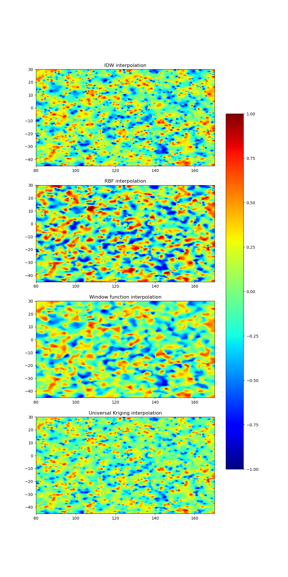
Let’s visualize our interpolated data

vmin = -1
vmax = 1
fig = matplotlib.pyplot.figure(figsize=(10, 20))
ax1 = fig.add_subplot(411)
pcm = ax1.pcolormesh(mx,
                     my,
                     idw,
                     cmap='jet',
                     shading='auto',
                     vmin=vmin,
                     vmax=vmax)
ax1.set_title('IDW interpolation')
ax2 = fig.add_subplot(412)
pcm = ax2.pcolormesh(mx,
                     my,
                     rbf,
                     cmap='jet',
                     shading='auto',
                     vmin=vmin,
                     vmax=vmax)
ax2.set_title('RBF interpolation')
ax3 = fig.add_subplot(413)
pcm = ax3.pcolormesh(mx,
                     my,
                     wf,
                     cmap='jet',
                     shading='auto',
                     vmin=vmin,
                     vmax=vmax)
ax3.set_title('Window function interpolation')
ax4 = fig.add_subplot(414)
pcm = ax4.pcolormesh(mx,
                     my,
                     kriging,
                     cmap='jet',
                     shading='auto',
                     vmin=vmin,
                     vmax=vmax)
ax4.set_title('Universal Kriging interpolation')
fig.colorbar(pcm, ax=[ax1, ax2, ax3, ax4], shrink=0.8)

<matplotlib.colorbar.Colorbar object at 0x7f5e964aaee0>