Geohash

Geohashing is a geocoding method used to encode geographic coordinates (latitude and longitude) into a short string of digits and letters delineating an area on a map, which is called a cell, with varying resolutions. The more characters in the string, the more precise the location.

Geohash Grid

import timeit

import cartopy.crs
import matplotlib.colors
import matplotlib.patches
import matplotlib.pyplot
import numpy
import pandas

#
import pyinterp

Writing a visualization routine for GeoHash grids.

def _sort_colors(colors):
    """Sort colors by hue, saturation, value and name in descending order."""
    by_hsv = sorted(
        (tuple(matplotlib.colors.rgb_to_hsv(matplotlib.colors.to_rgb(color))),
         name) for name, color in colors.items())
    return [name for hsv, name in reversed(by_hsv)]


def _plot_box(ax, code, color, caption=True):
    """Plot a GeoHash bounding box."""
    box = pyinterp.GeoHash.from_string(code.decode()).bounding_box()
    x0 = box.min_corner.lon
    x1 = box.max_corner.lon
    y0 = box.min_corner.lat
    y1 = box.max_corner.lat
    dx = x1 - x0
    dy = y1 - y0
    box = matplotlib.patches.Rectangle((x0, y0),
                                       dx,
                                       dy,
                                       alpha=0.5,
                                       color=color,
                                       ec='black',
                                       lw=1,
                                       transform=cartopy.crs.PlateCarree())
    ax.add_artist(box)
    if not caption:
        return
    rx, ry = box.get_xy()
    cx = rx + box.get_width() * 0.5
    cy = ry + box.get_height() * 0.5
    ax.annotate(code.decode(), (cx, cy),
                color='w',
                weight='bold',
                fontsize=16,
                ha='center',
                va='center')


def plot_geohash_grid(precision,
                      polygon=None,
                      caption=True,
                      color_list=None,
                      inc=7):
    """Plot geohash bounding boxes."""
    color_list = color_list or matplotlib.colors.CSS4_COLORS
    fig = matplotlib.pyplot.figure(figsize=(24, 12))
    ax = fig.add_subplot(1, 1, 1, projection=cartopy.crs.PlateCarree())
    if polygon is not None:
        box = polygon.envelope() if isinstance(
            polygon, pyinterp.geodetic.Polygon) else polygon

        ax.set_extent(
            [
                box.min_corner.lon,
                box.max_corner.lon,
                box.min_corner.lat,
                box.max_corner.lat,
            ],
            crs=cartopy.crs.PlateCarree(),
        )
    else:
        box = None
    colors = _sort_colors(color_list)
    ic = 0
    codes = pyinterp.geohash.bounding_boxes(polygon, precision=precision)

    color_codes = {codes[0][0]: colors[ic]}
    for item in codes:
        prefix = item[precision - 1]
        if prefix not in color_codes:
            ic += inc
            color_codes[prefix] = colors[ic % len(colors)]
        _plot_box(ax, item, color_codes[prefix], caption)
    ax.stock_img()
    ax.coastlines()
    ax.grid()

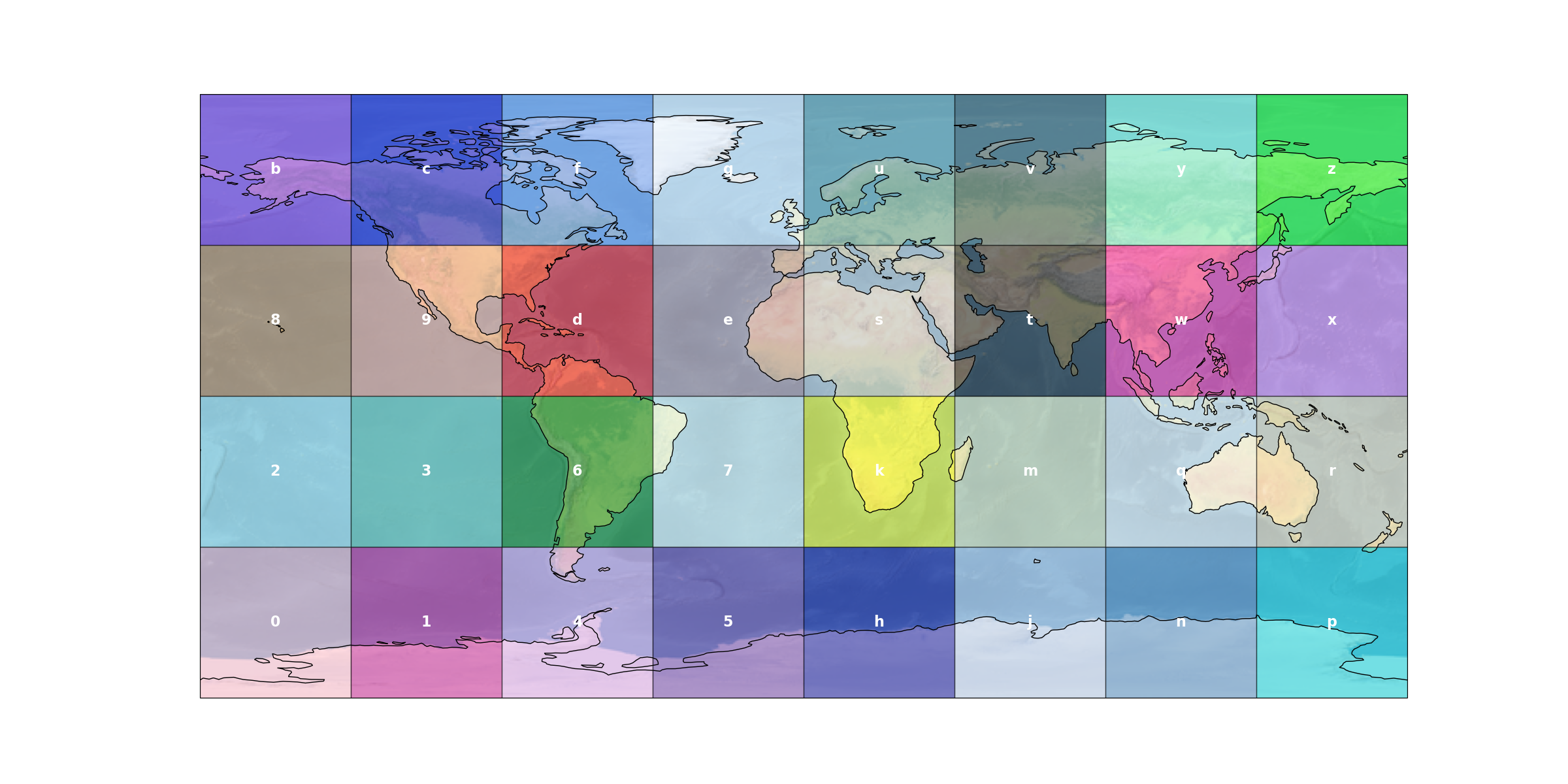
Bounds of geohash with a precision of 1 character.

plot_geohash_grid(1)

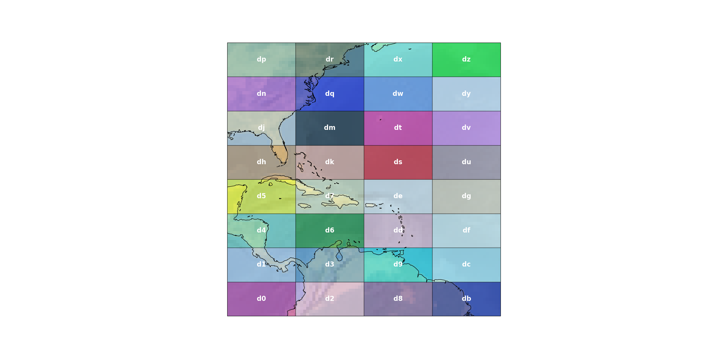
Bounds of the geohash d with a precision of two characters.

plot_geohash_grid(2, polygon=pyinterp.GeoHash.from_string('d').bounding_box())

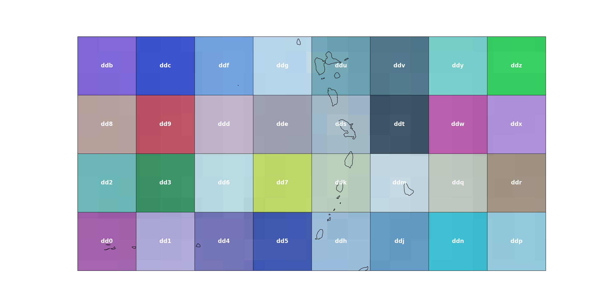
Bounds of the geohash dd with a precision of three characters.

plot_geohash_grid(3, polygon=pyinterp.GeoHash.from_string('dd').bounding_box())

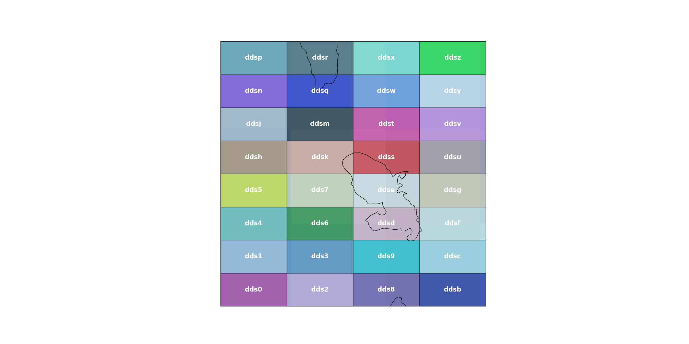
Bounds of the geohash dds with a precision of four characters.

plot_geohash_grid(4,
                  polygon=pyinterp.GeoHash.from_string('dds').bounding_box())

The GeoHash class allows encoding a coordinate into a GeoHash code in order to examine its properties: precision, number of bits, code, coordinates of the grid cell, etc.

code = pyinterp.GeoHash(-67.5, 22.5, precision=4)
print(f'code = {code!s})')
print(f'precision = {code.precision()}')
print(f'number of bits = {code.number_of_bits()}')
print(f'lon/lat = {code.center()}')

code = ds00)
precision = 4
number of bits = 20
lon/lat = (-67.3242, 22.5879)

You can also use this class to get the neighboring GeoHash codes of this instance.

[str(item) for item in code.neighbors()]

# On the other hand, when you want to encode a large volume of data, you should
# use functions that work on numpy arrays.

['ds01', 'ds03', 'ds02', 'debr', 'debp', 'd7zz', 'dkpb', 'dkpc']

Encoding coordinates

Generation of dummy data

SIZE = 1000000
lon = numpy.random.uniform(-180, 180, SIZE)
lat = numpy.random.uniform(-80, 80, SIZE)
measures = numpy.random.random_sample(SIZE)

Encoding the data

codes = pyinterp.geohash.encode(lon, lat, precision=4)
codes

# As you can see, the resulting codes are encoding as numpy byte arrays.

array([b'4rxm', b'0v5v', b'dhw7', ..., b'71t5', b'0zrb', b's3e2'],
      dtype='|S4')

This algorithm is very fast, which makes it possible to process a lot of data quickly.

timeit.timeit('pyinterp.geohash.encode(lon, lat)',
              number=50,
              globals=dict(pyinterp=pyinterp, lon=lon, lat=lat)) / 50

0.03452457465999942

The inverse operation is also possible.

lon, lat = pyinterp.geohash.decode(codes)

You can also use the pyinterp.geohash.transform() to transform coordinates from one précision to another.

codes = pyinterp.geohash.transform(codes, precision=1)
codes

array([b'0', b'1', b'2', b'3', b'4', b'5', b'6', b'7', b'8', b'9', b'b',
       b'c', b'd', b'e', b'f', b'g', b'h', b'j', b'k', b'm', b'n', b'p',
       b'q', b'r', b's', b't', b'u', b'v', b'w', b'x', b'y', b'z'],
      dtype='|S1')

codes = pyinterp.geohash.transform(codes, precision=3)
codes

array([b'000', b'001', b'004', ..., b'zzv', b'zzy', b'zzz'], dtype='|S3')

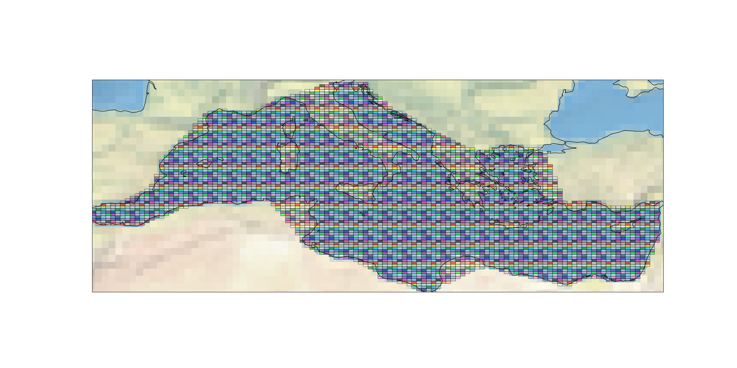
The pyinterp.geohash.bounding_boxes() function allows calculating the GeoHash codes contained in a box or a polygon. This function allows, for example, to obtain all the GeoHash codes present on the Mediterranean.

MEDITERRANEAN_SEA = [(-1.43504, 35.38124), (-1.68901, 35.18381),
                     (-1.93947, 35.18664), (-2.18994, 35.18945),
                     (-2.44041, 35.19223), (-2.69089, 35.19498),
                     (-3.19185, 35.20043), (-3.44234, 35.20312),
                     (-4.19382, 35.21103), (-4.44432, 35.21363),
                     (-4.69483, 35.21619), (-4.94221, 35.42047),
                     (-5.18954, 35.62438), (-5.18619, 35.82515),
                     (-5.18272, 36.02538), (-5.17911, 36.22509),
                     (-4.92467, 36.42114), (-4.41929, 36.61311),
                     (-4.16856, 36.60978), (-3.91785, 36.60641),
                     (-3.66714, 36.60302), (-3.41643, 36.59959),
                     (-1.64252, 37.35734), (-0.61682, 38.11193),
                     (-0.05974, 39.61617), (-0.05188, 39.80296),
                     (0.47608, 40.34624), (1.0068, 40.88237),
                     (1.26823, 41.05687), (3.17405, 43.12814),
                     (3.95946, 43.44167), (4.21176, 43.4303),
                     (4.46402, 43.41885), (5.4578, 43.20103),
                     (7.00043, 43.46998), (7.2684, 43.62615),
                     (8.32692, 44.07445), (8.59664, 44.22593),
                     (8.86679, 44.37629), (9.11878, 44.36187),
                     (12.30323, 45.45208), (12.82897, 45.57254),
                     (13.35502, 45.69103), (13.60653, 45.6726),
                     (14.56628, 45.29165), (14.77339, 44.96545),
                     (16.35039, 43.4468), (16.83351, 43.25904),
                     (17.31681, 43.07169), (18.26742, 42.54036),
                     (18.50146, 42.36803), (18.73581, 42.19562),
                     (19.45557, 41.83742), (22.59567, 40.39801),
                     (23.86967, 40.66103), (24.38198, 40.79528),
                     (25.14395, 40.91539), (25.39346, 40.90312),
                     (25.87922, 40.72341), (27.3756, 40.65146),
                     (27.3629, 40.4972), (27.35049, 40.34214),
                     (28.89327, 36.67855), (30.6478, 36.80647),
                     (30.89745, 36.80017), (31.14709, 36.79388),
                     (31.63983, 36.61137), (32.1328, 36.42873),
                     (34.38535, 36.54538), (34.64117, 36.70704),
                     (34.89068, 36.70094), (35.89499, 36.84229),
                     (36.14443, 36.83607), (36.13812, 36.67067),
                     (35.84461, 35.31519), (35.83989, 35.14037),
                     (35.83535, 34.96453), (35.83096, 34.78764),
                     (35.82673, 34.60973), (35.82266, 34.43077),
                     (35.56521, 34.07323), (35.30493, 33.52656),
                     (35.04582, 32.96983), (34.78535, 32.21131),
                     (34.53086, 31.82665), (34.27678, 31.43758),
                     (34.02492, 31.24227), (33.77499, 31.24401),
                     (33.52506, 31.24576), (33.27513, 31.24751),
                     (33.02519, 31.24927), (32.77526, 31.25102),
                     (32.52532, 31.25279), (32.27538, 31.25455),
                     (30.52777, 31.46553), (29.27227, 30.87518),
                     (29.0223, 30.87679), (28.27422, 31.08288),
                     (27.52624, 31.28865), (26.5284, 31.49606),
                     (25.53067, 31.70343), (25.28069, 31.70546),
                     (24.03548, 32.11364), (23.28805, 32.31846),
                     (20.02259, 30.93524), (19.77083, 30.7316),
                     (19.51917, 30.52699), (19.26761, 30.32143),
                     (19.01759, 30.32277), (18.51909, 30.5327),
                     (17.77237, 30.94967), (17.0241, 31.15993),
                     (16.02586, 31.37173), (15.77581, 31.37348),
                     (15.52992, 31.78362), (13.79181, 32.80886),
                     (12.7914, 32.81862), (12.54129, 32.82104),
                     (12.04387, 33.02684), (11.54655, 33.23236),
                     (10.30532, 33.84446), (10.05858, 34.04584),
                     (10.06218, 34.24361), (7.87667, 36.9875),
                     (7.12516, 37.00275), (6.87464, 37.00779),
                     (5.86671, 36.83664), (5.61618, 36.84139),
                     (5.36563, 36.84612), (5.11508, 36.85081),
                     (4.86453, 36.85549), (3.61163, 36.87846),
                     (2.60396, 36.70273), (2.35336, 36.70699),
                     (1.34599, 36.52884), (0.07965, 35.95831),
                     (-0.67601, 35.77038), (-1.43504, 35.38124)]
polygon = pyinterp.geodetic.Polygon(
    [pyinterp.geodetic.Point(lon, lat) for lon, lat in MEDITERRANEAN_SEA])

precision = 4
plot_geohash_grid(precision, polygon=polygon, caption=False)

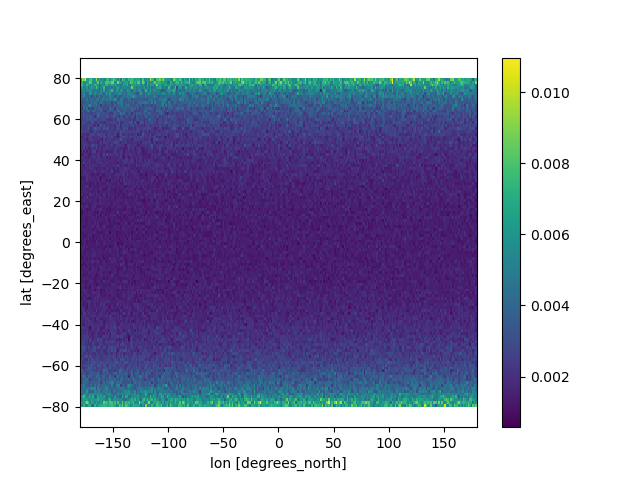
Density calculation

df = pandas.DataFrame(
    dict(lon=lon,
         lat=lat,
         measures=measures,
         geohash=pyinterp.geohash.encode(lon, lat, precision=3)))
df.set_index('geohash', inplace=True)
df = df.groupby('geohash').count()['measures'].rename('count').to_frame()
df['density'] = df['count'] / (
    pyinterp.geohash.area(df.index.values.astype('S')) / 1e6)
array = pyinterp.geohash.to_xarray(df.index.values.astype('S'), df.density)
array = array.where(array != 0, numpy.nan)

fig = matplotlib.pyplot.figure()
ax = fig.add_subplot(111)
_ = array.plot(ax=ax)