4D interpolation

Interpolation of a four-dimensional regular grid.

Quadrivariate

The quadrivariate interpolation allows obtaining values at arbitrary points in a 4D space of a function defined on a grid.

This method performs a bilinear interpolation in 2D space by considering the axes of longitude and latitude of the grid, then performs a linear interpolation in the third and fourth dimensions. Its interface is similar to the trivariate class except for a fourth axis, which is handled by this object.

import cartopy.crs
import matplotlib
import matplotlib.pyplot
import numpy

import pyinterp
import pyinterp.backends.xarray
import pyinterp.tests

The first step is to load the data into memory and create the interpolator object:

ds = pyinterp.tests.load_grid4d()
interpolator = pyinterp.backends.xarray.Grid4D(ds.pressure)

We will build a new grid that will be used to build a new interpolated grid.

Warning

When using a time axis, care must be taken to use the same unit of dates, between the axis defined and the dates supplied during interpolation. The function pyinterp.TemporalAxis.safe_cast() automates this task and will warn you if there is an inconsistency during the date conversion.

mx, my, mz, mu = numpy.meshgrid(numpy.arange(-125, -70, 0.5),
                                numpy.arange(25, 50, 0.5),
                                numpy.datetime64('2000-01-01T12:00'),
                                0.5,
                                indexing='ij')

We interpolate our grid using a classical:

quadrivariate = interpolator.quadrivariate(
    dict(longitude=mx.ravel(),
         latitude=my.ravel(),
         time=mz.ravel(),
         level=mu.ravel())).reshape(mx.shape)

Bicubic on 4D grid

Used grid organizes the latitudes in descending order. We ask our constructor to flip this axis in order to correctly evaluate the bicubic interpolation from this 4D cube (only necessary to perform a bicubic interpolation).

interpolator = pyinterp.backends.xarray.Grid4D(ds.pressure,
                                               increasing_axes=True)

We interpolate our grid using a bicubic interpolation in space followed by a linear interpolation in the temporal axis:

bicubic = interpolator.bicubic(dict(longitude=mx.ravel(),
                                    latitude=my.ravel(),
                                    time=mz.ravel(),
                                    level=mu.ravel()),
                               nx=2,
                               ny=2).reshape(mx.shape)

We transform our result cubes into a matrix.

quadrivariate = quadrivariate.squeeze(axis=(2, 3))
bicubic = bicubic.squeeze(axis=(2, 3))
lons = mx[:, 0].squeeze()
lats = my[0, :].squeeze()

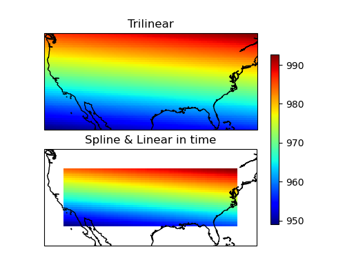
Let’s visualize our results.

Note

The resolution of the grid example is very low (one pixel everyone degree) therefore the calculation window cannot find the required pixels at the edges to calculate the interpolation correctly. See Chapter Fill NaN values to see how to address this issue.

fig = matplotlib.pyplot.figure(figsize=(5, 4))
ax1 = fig.add_subplot(
    211, projection=cartopy.crs.PlateCarree(central_longitude=180))
pcm = ax1.pcolormesh(lons,
                     lats,
                     quadrivariate.T,
                     cmap='jet',
                     shading='auto',
                     transform=cartopy.crs.PlateCarree())
ax1.coastlines()
ax1.set_title('Trilinear')

ax2 = fig.add_subplot(
    212, projection=cartopy.crs.PlateCarree(central_longitude=180))
pcm = ax2.pcolormesh(lons,
                     lats,
                     bicubic.T,
                     cmap='jet',
                     shading='auto',
                     transform=cartopy.crs.PlateCarree())
ax2.coastlines()
ax2.set_title('Spline & Linear in time')
fig.colorbar(pcm, ax=[ax1, ax2], shrink=0.8)
fig.show()